
PG Phriday: When Partitioning Goes Wrong
I’ve been talking about partitions a lot recently, and I’ve painted them in a very positive light. Postgres partitions are a great way to distribute data along a logical grouping and work best when data is addressed in a fairly isloated manner. But what happens if we direct a basic query at a partitioned table in such a way that we ignore the allocation scheme? Well, what happens isn’t pretty. Let’s explore in more detail.
Let’s use the fancy partitioning I introduced a while back. Using this structure, I ran a bunch of tests with a slight modification to my python script. I changed the reading_date granularity to daily, and had the script itself create and destroy the partitions. This allowed me to run several iterations and then meter the performance of queries on the resulting output.
The relevant python chunk looks like this:
end_stamp = stamp + timedelta(days = 1)

part = ''
if j > 0:
    part = '_part_%d%02d%02d' % (stamp.year, stamp.month, stamp.day)

    cur.execute("DROP TABLE IF EXISTS sensor_log%s" % part)

    cur.execute(
      "CREATE TABLE sensor_log%s (" % part +
      "LIKE sensor_log INCLUDING ALL," +
      "  CHECK (reading_date >= '%s' AND" % stamp.date() +
      "    reading_date < '%s')" % end_stamp.date() +
      ") INHERITS (sensor_log)"
    )

    db_conn.commit()
With that, the script will assume daily granularity and build the check constraints properly so constraint exclusion works as expected. To get an idea of how partitions scale with basic queries, I ran the script with 10, 20, 50, 100, 150, and 250 days. This gave a wide distribution of partition counts and the numbers I got made it fairly clear what kind of drawbacks exist.
All tests on the partition sets used these two queries:
-- Check 100 distributed values in the partitions.
EXPLAIN ANALYZE
SELECT *
  FROM sensor_log
 WHERE sensor_log_id IN (
         SELECT generate_series(1, 10000000, 100000)
       );

-- Check 100 random values in the partitions.
EXPLAIN ANALYZE
SELECT *
  FROM sensor_log
 WHERE sensor_log_id IN (
         SELECT (random() * 10000000)::INT
           FROM generate_series(1, 100)
       );
The goal of these queries is to stress the query planner. I’ve omitted the reading_date column entirely so no partitions can be excluded. Since the primary key isn’t how the tables are grouped, a random assortment of keys must be retrieved from all partitions.
Thinking upon this for a moment, we might expect a linear increase in query execution time by partition count. The reason for that is fairly simple: each child partition is addressed independently. But we also need to take the query planner itself into account. As the amount of partitions increase, so does the amount of potential query plans.
Do the tests bare that out? These are the results obtained from a VM. All times are in milliseconds, and in every case, the entry is the best time obtained, not an average.
| Partitions | Plan 1 | Exec 1 | Plan 2 | Exec 2 | Diff Plan | Diff Exec |
|---|---|---|---|---|---|---|
| 1 | 0.151 | 0.450 | 0.174 | 0.480 | N/A | N/A |
| 10 | 0.539 | 2.298 | 0.753 | 2.816 | 4.0 | 5.5 |
| 20 | 0.890 | 4.655 | 1.384 | 5.006 | 6.9 | 10.4 |
| 50 | 2.320 | 13.712 | 2.207 | 14.120 | 14.0 | 30.0 |
| 100 | 6.050 | 32.822 | 6.777 | 41.311 | 39.5 | 79.5 |
| 150 | 10.088 | 48.535 | 10.594 | 52.406 | 63.8 | 108.5 |
| 250 | 24.267 | 81.278 | 28.226 | 81.618 | 161.5 | 168.3 |
If we examine the contents of this table, a few things pop out. First, partitions definitely decrease performance when the partitioned column isn’t included in the query. We already knew that, so what else is there? I averaged the difference of execution times for both query plans and the queries themselves to represent the degree of slowdown. Here’s a graph of just the last two columns:
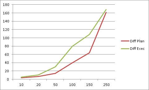
There is some variance, but the degree of slowdown is not linear. As the number of partitions increase, the divergence from baseline accelerates. Further, it appears there’s an arbitrary point where the planner just falls apart. A more in-depth analysis could probably reveal when that happens for these queries, but it would be different for others. In either case, ten partitions is about four times slower than ideal, so 25x more partitions should result in a plan time of 100ms—which is 60% less than what we actually observed. At 150, we’d expect 60ms, and measurements are pretty close to that value.
What this means in the long run is that query plans cost time. As the number of partitions grows, we should expect planning time to rise faster. Times are also additive. So at 100 partitions, total query time is actually about 60x slower than no partitions at all.
The lesson here isn’t to avoid Postgres partitions entirely, but to use them sparingly and in ideal circumstances. If data can’t be delineated along specific groupings and addressed by individual segment, it should not be partitioned. In other words, if the column used to split up the data isn’t in almost every query, it’s probably the wrong approach.
There is of course, a caveat to that statement: parallelism can address part of this problem. Postgres developers have been working hard on adding parallelism to the base engine, and partitions are a natural target. It would seem possible to launch a separate backend process to obtain data from each segment independently, and aggregate it at the end. This would massively reduce query execution time, but query planning time would likely increase to accommodate the extra functionality.
Yet I’ve heard people are looking into fixing how the planner handles partitions, so that too could eventually decrease substantially. In the end, I stand by partitions simply because they’re useful, and I’ll continue to recommend them. But like all tasty things, this should come with a grain of salt; it’s easy to partition something that shouldn’t be, or do so on the wrong vector, and suffer the consequences.